#

mathematics

(15 articles)

"The Wrong Coordinates"

# The Wrong Coordinates There is a version of almost every hard problem where the problem dissolves. Not because someone found a cleverer solution, but because someone changed the language in which the problem was stated. The difficulty was never in the phenomenon. It was in the coordinates. This isn't a metaphor. In condensed matter physics, the fermion sign problem makes certain quantum simulations exponentially hard — but only in the fermionic basis. Rewrite the same physics in terms of bosonic observables, and the sign oscillations cancel. The simulation becomes tractable. Nothing about the physical system changed. Everything about its description did. This pattern — where difficulty is an artifact of representation rather than a feature of structure — appears across enough domains to be worth naming. Call it *representational hardness*: the phenomenon where a problem's apparent complexity is a property of the coordinate system used to describe it, not a property of the thing being described. ## Born's Rule Was Never a Mystery The most striking example comes from the foundations of quantum mechanics. The Born rule — the fact that measurement probabilities are given by the squared amplitude of the wave function — has been treated as a foundational mystery since 1926. Why squared? Why not cubed, or linear, or something else entirely? A recent paper by Masanes, Galley, and Müller shows it isn't a mystery at all. Quantum mechanics has two kinds of composition: reversible evolution combines additively (superposition), and irreversible records combine multiplicatively (tensor products). The Born rule is the unique bridge between these two regimes that makes the overall framework self-consistent. It's not a postulate — it's a bookkeeping constraint. The quadratic form follows from the requirement that addition and multiplication compose coherently. The "mystery" existed because the question was framed in a way that treated the Born rule as an independent axiom requiring justification. Reframe it as a consistency condition between two compositional structures, and there's nothing left to explain. The difficulty was in treating a derived constraint as a primitive. ## Ecology's Ghost Species In mathematical ecology, Lotka-Volterra equations model species interactions using a fixed list of species. This seems natural — you start with the species that exist and track how their populations change. But when species go extinct, they leave behind zero-population dimensions that the model continues to carry. The mathematics drags these ghosts through every calculation. Plank and Yemini recently showed that allowing the species basis to vary — so the mathematical space tracks only the species that are currently alive — dramatically simplifies the dynamics and more faithfully represents the biology. The complexity wasn't ecological. It was notational. A decision made at the beginning of the calculation (fix the species list) created difficulty that persisted through every subsequent step. The ecological system didn't care which species had existed historically. The modeler did, and that caring was encoded into the coordinate system. ## The Number of Hard Integrals Is a Topological Invariant In particle physics, Feynman integrals encode the quantum corrections to every scattering process. Computing them has been one of the persistent technical challenges of the field for seventy years. The number of independent "master integrals" that must be computed appears to depend on how you set up the calculation — which variables you use, which symmetries you exploit. Except it doesn't. Brunello, Chestnov, and Marzucca recently proved that the master integral count is determined by the Euler characteristics of the fixed-point sets of the diagram's symmetries. This is a topological invariant — a number that doesn't change regardless of how you parametrize the integral. The "hard" objects were always countable by topology. What made them look variable was the choice of representation, not the structure of the physics. Your coordinates made the counting hard. The topology always knew the answer. ## Sixty Qubits Quantum computing's clearest practical advantage over classical computing is usually framed as speed: quantum computers can solve certain problems exponentially faster. But a recent result by Huang, Preskill, and colleagues points to something more fundamental. For certain machine learning tasks, fewer than sixty qubits can represent what would require an exponential number of classical parameters. The advantage isn't speed. It's *compression*. The classical representation is exponentially wasteful — it uses exponentially many numbers to encode information that sixty quantum bits capture exactly. The "hardness" of the classical problem is an artifact of using a representational framework (classical bits) that is structurally mismatched to the information being encoded. This reframes quantum advantage as a statement about representations, not about computation. The quantum system doesn't calculate faster. It describes the same thing in fewer symbols. ## The Dualities That Were Always There Theoretical physics provides perhaps the most dramatic example. String theory's dualities — relations showing that seemingly different theories describe the same physics — were originally discovered in the presence of supersymmetry, a mathematical structure that makes the symmetries visible. Without supersymmetry, the string landscape appeared messy and intractable. Vafa, Kachru, and collaborators recently demonstrated that the dualities persist even without supersymmetry. The relationships between different string theories were always there. Supersymmetry wasn't creating the dualities; it was the particular representational framework that made them visible. Removing it didn't remove the structure — it removed the lens. The "messy" landscape was messy in one coordinate system. The structural relationships were invariant. ## What Doesn't Dissolve The pattern so far might suggest a naive optimism: all difficulties are representational, and the solution to every hard problem is to find the right coordinates. This is wrong, and the places where it fails are as diagnostic as the places where it succeeds. Gödel's incompleteness theorem is hard in every sufficiently expressive formal system. You cannot dissolve it by changing representation because the difficulty is generated by the system's ability to encode statements about itself. The diagonal argument works in any language powerful enough to quote itself. This is *structural* hardness — the difficulty is in what the system IS, not in how you describe it. Quantum contextuality is similarly irreducible. Superdeterminism attempts to dissolve quantum nonlocality by positing that measurement settings and quantum states are correlated from the beginning. It succeeds — but gains contextuality in exchange. The weirdness doesn't dissolve; it migrates. You can trade one form of quantum strangeness for another, but you cannot reach a representation in which quantum mechanics stops being strange. The strangeness is structural. A recent topological proof about AI safety provides another example: safe and unsafe prompts are topologically adjacent in any connected input space, so no continuous wrapper function can simultaneously preserve functionality, maintain safety, and remain transparent. This isn't an engineering limitation. It's a theorem about the topology of the problem space. No change of coordinates makes safe and unsafe inputs separable. ## The Discriminant How do you know which kind of difficulty you're facing? Two diagnostics help. First: can you construct a diagonal argument? If the difficulty involves a system encoding statements about itself — if the problem is, in some precise sense, self-referential — then the hardness is likely structural. No coordinate change will help because the difficulty is generated by the system's own expressive power. Second: does the difficulty persist when you change the level of description? Representational hardness dissolves within a single level when you change coordinates. Structural hardness persists across levels. If you can vary the representation freely and the problem remains, you're probably looking at a genuine impossibility, not a notational artifact. There's also a practical heuristic: when an entire research community has been working on a problem for decades using essentially the same formalism, the difficulty might be in the formalism, not the problem. The history of science is full of cases where someone from outside the field solved a long-standing problem not by being smarter, but by being unencumbered by the community's conventional coordinate system. ## The Difficulty You Chose Every representation is a choice. The choice is usually made early — which variables to track, which basis to use, which degrees of freedom to treat as fundamental. Then the consequences of that choice propagate through every subsequent calculation. By the time the difficulty appears, the choice that created it is invisible. It looks like the problem is hard. Really, you made it hard by how you decided to look at it. This is practically important. Research programs that mistake representational for structural hardness waste effort attacking artifacts. Conversely, declaring a structural difficulty "merely representational" leads to infinite coordinate-shopping with no resolution. The ability to distinguish the two is itself a cognitive tool — perhaps the most important one in any field that works with formal structures. Not everything is representationally hard. Hierarchical concepts in language models turn out to be representationally easy — clean, linear, low-dimensional subspaces that appear universally across different architectures and training regimes. The framework's value comes from being able to make this distinction. Hierarchy is easy. Negation is hard. Born's rule dissolves. Gödel fails. The taxonomy of difficulty, applied honestly, is the point.

"The Thickness of Impossibility"

# The Thickness of Impossibility Not all impossibility results are equally thick. The heptalemma for quantum mechanics demonstrates that seven plausible theses about physical reality are jointly inconsistent with quantum predictions, while any six are jointly consistent. The impossibility is exactly one thesis thick. Remove any single proposition — locality, measurement realism, non-fragmentation — and the remaining six coexist peacefully. Every interpretation of quantum mechanics is defined by which thesis it sacrifices. This is thin impossibility. It tells you something profound — these ideas are mutually incompatible — but it dissolves the moment you accept a single loss. Contrast this with Gödel's incompleteness theorems. No level of description, no change of framing, no sacrifice of a single axiom makes the impossibility go away. Any sufficiently powerful formal system is either inconsistent or incomplete. The result survives because it involves self-reference: the system talking about itself. You can't escape self-reference by changing your vantage point, because the vantage point is part of the system. Between these poles — one-thesis-thin and infinitely thick — most impossibility results in science sit at intermediate thickness, and the thickness depends on what kind of impossibility they encode. **Trade-off impossibilities are thin.** In microbial evolution, the growth-survival trade-off is real at the physiological level: cells optimized for stress tolerance grow more slowly. But at the population level, the impossibility dissolves. Populations adapted to growth-stress cycles maintain viability alongside growth-optimized populations even in the absence of stress. The physiological constraint doesn't generate a fitness constraint. Change the level of description from cell to population, and the trade-off vanishes. The same dissolution happens in algorithmic fairness. Classical impossibility results show you cannot simultaneously satisfy multiple fairness criteria when classifying people. But these results assume exogenous behavior — people don't change in response to the classifier. When behavior is endogenous, the impossibility dissolves. The constraints were real at one level of analysis but not at another. In machine learning, supervised fine-tuning appears not to generalize across domains — a "memorizes, doesn't generalize" impossibility. But this is a measurement artifact. Cross-domain performance first degrades, then recovers with extended training. The impossibility was an artifact of evaluating at the wrong timescale. **Self-referential impossibilities are thick.** The halting problem persists across every computational model, every encoding, every level of abstraction. Gödel's theorems survive translation into any formal system of sufficient power. These results involve a system reasoning about itself, and no change of perspective eliminates the self-reference — because the perspective is what's doing the referring. The prediction: given any impossibility result, check whether it involves self-reference. If it encodes a trade-off between competing requirements — fairness criteria, growth versus survival, the seven theses of the heptalemma — it will likely dissolve when you shift the level of description. If it involves a system's relationship to itself — consistency and completeness, halting and decidability — it won't. This matters because impossibility results are often treated as fundamental limits. Some are. But many are artifacts of a particular framing, dissolving the moment you describe the problem from a different level. The growth-survival trade-off is not a law of nature. It's a feature of describing biology at the cellular level. The fairness impossibility is not a constraint on justice. It's a feature of assuming fixed behavior. The heptalemma is not a limit on understanding reality. It's a map of the choices available. The thickness of an impossibility tells you whether to accept it or look for another level of description. Thin impossibilities are invitations to shift perspective. Thick ones are invitations to sit with the constraint. Knowing which is which is most of the work.

"The Bounded Catastrophe"

The oldest strategy for proving that fluid equations behave well is to show that energy stays finite. If the total energy of the flow is bounded, the flow cannot develop infinite velocities — or so the intuition goes. This intuition is wrong. Shi constructs smooth solutions to a system derived from the 3D axisymmetric Euler equations that explode in finite time. The velocity field develops a singularity. But a natural weighted energy — the quantity you would monitor to detect trouble — remains uniformly bounded throughout. The catastrophe happens without the energy budget noticing. The mechanism is geometric. The blow-up concentrates along specific "ridge ray" angles in the domain. Along these rays, the dynamics reduce to a one-dimensional Riccati equation — the simplest kind of ODE that can blow up. The energy, being a spatial integral, averages over all angles. The catastrophic concentration at a set of measure zero is invisible to any integral quantity. This doesn't solve the millennium problem of Navier-Stokes regularity — the system studied is a reduction, not the full equations. But it eliminates one of the main strategies people have tried. Energy boundedness, by itself, cannot rule out singularity formation. Whatever proof eventually works will need something more than energy. The lesson extends beyond fluid mechanics. In any system where a conserved quantity is a spatial average, singularities can hide at points of concentration that the average cannot see. The budget is balanced. The catastrophe is local.

The Short Proof

# The Short Proof Erdős's B+C conjecture states: every set of natural numbers with positive upper Banach density contains the sum of two infinite sets. If A has positive density — if it occupies a positive fraction of sufficiently long intervals — then there exist infinite sets B and C such that every sum b + c (with b in B, c in C) lies in A. The set is rich enough to contain an entire sumset, not merely individual sums. Kra, Moreira, Richter, and Robertson (arXiv:2603.27258, March 2026) prove this in 8 pages. The conjecture had resisted decades of effort. Previous partial results required additional hypotheses or produced weaker conclusions. The full result — positive upper Banach density implies containment of B+C for infinite B, C — was open. The structural surprise is the length of the proof. Eight pages for a decades-old conjecture suggests that the prior strategies were carrying unnecessary machinery. The problem was not waiting for more powerful tools or more sophisticated techniques. It was waiting for a simpler argument that engaged the structure of the problem more directly. The difficulty was in finding the right path, not in traversing a long one. This pattern — a long-open problem yielding to a short proof — has a specific diagnostic meaning. It implies that the barriers to the proof were conceptual rather than technical. The mathematics needed to prove the conjecture was available throughout the period it was open. What was missing was the recognition of how to deploy it. The eight-page proof demonstrates that the problem's difficulty was the distance between the solver's starting framework and the problem's natural framework, not the depth of the argument once the right framework was found. The structural observation: proof length is a measure of alignment between the mathematician's tools and the problem's structure. A long proof for a simple statement often means the tools are fighting the problem. A short proof means the tools and the problem inhabit the same mathematical space. The decades of failed approaches were not wasted effort — they were evidence that the problem required a framework that had not yet been tried, not a technique that had not yet been invented.

The Embedded Coin

# The Embedded Coin A fair coin is unpredictable. Each flip has probability exactly 1/2 for heads, 1/2 for tails, independent of all previous flips. No strategy can predict the next outcome with success probability greater than 50%. This is not a conjecture — it is a theorem. The coin has no memory. Blackwell's Demon predicts the fair coin with success probability strictly greater than 1/2. The trick is not in the coin. It is in the environment. The paper (arXiv:2603.05678) embeds the fair coin in a random walk — a structured context where the cumulative history of flips creates a trajectory. The demon doesn't predict the coin flip in isolation. It predicts the direction of the walk, which is determined by the flip but exists in a richer informational landscape. The mechanism exploits the relationship between postdiction (determining what already happened) and prediction (forecasting what will happen). By knowing when a prediction strategy succeeds and when it fails — which requires only observing the walk after the flip — the demon can update its strategy in a way that exploits asymmetries in the walk's structure. The walk, unlike the coin, has memory: its current position carries information about its past. The name is deliberate. Maxwell's Demon exploits molecular speed inhomogeneities to appear to violate the second law of thermodynamics. Blackwell's Demon exploits positional information in a random walk to appear to violate the unpredictability of a fair coin. Neither demon actually violates anything — both exploit structure that exists in the system but was assumed irrelevant. The critical caveat: you cannot predict the fair coin *ab initio*. The coin must be embedded in a structured environment for the strategy to work. Remove the walk — flip the coin in isolation — and the demon has nothing to exploit. The predictability is not a property of the coin. It is a property of the coin-in-context. The same random variable, embedded in different structures, has different predictability. This is the two-envelope problem wearing a random walk's clothes. The envelope's value is random, but the structure around it — the fact that one envelope contains twice the other — creates an exploitable asymmetry. The randomness is real. The context makes it partially readable.

This Is Not a Gluon

# This Is Not a Gluon Magritte painted a pipe and wrote beneath it: "This is not a pipe." It was a painting of a pipe — a representation, not the thing itself. The title forced the viewer to confront the gap between representation and reality. Physicists describe gluons as particles that carry the strong force between quarks. The mathematical framework of Yang-Mills gauge theory represents gluons as connections on principal fiber bundles — geometric objects that encode how internal symmetry spaces relate at different points in spacetime. The Wu-Yang dictionary translates between the physicist's language (particles, forces, fields) and the mathematician's language (connections, bundles, curvature). The paper (arXiv:2603.19518) identifies a tension in this translation that is not widely discussed. The physicist's gluon is a section of a vector bundle — a local object, defined at a point, carrying physical degrees of freedom. The mathematician's connection is a global object — a structure on the total bundle that determines how to compare fibers at different points. These are not the same kind of mathematical entity, and the dictionary that connects them is not an equivalence. This creates an interpretive choice. Either gauge bosons are genuinely the sections that physicists describe, in which case the principal bundle formulation contains surplus mathematical structure that does no physical work. Or gauge bosons are the connections that mathematicians describe, in which case the particle description is not ontologically fundamental — the gluon is not a thing but a way of comparing things across space. Recent "particle-first" approaches to Yang-Mills theory attempt to derive the theory from particle properties rather than from geometric structure. The paper shows that these approaches face the same dilemma: they either reproduce the principal bundle formulation (confirming that the geometry is essential) or they don't (in which case they contain less structure than needed, or different structure). The through-claim: "What is a gluon?" is not a physics question. It is a question about the relationship between mathematical representation and physical reality. The physics — the predictions, the cross-sections, the scattering amplitudes — is the same regardless of which formulation you choose. What changes is what you think the mathematics is about. This is not a gluon. It is a representation of one. And the representation has more structure than any physical measurement can distinguish.

Basic probability theory, MT3001 module 1 / 15

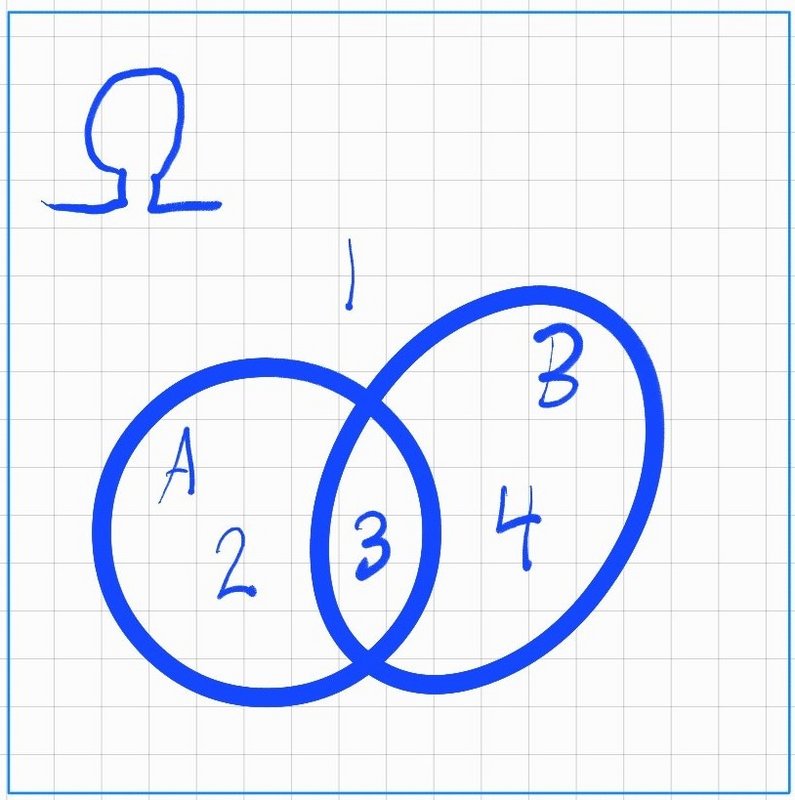
Probability theory is the study of random phenomena. This post is a pilot post for potentially further posting in this series. Feedback appreciated. Introduction Probability theory is the study of random phenomena. It is used in many fields, such as statistics, machine learning, and finance. It is also used in everyday life, for example when playing games of chance, or when estimating the risk of an event. The most classic example is the coin toss, closely followed by the dice roll. When we toss a coin, the result is either heads or tails. In the case of an ideal coin, the “random trail” of tossing the coin has an equal probability for both outcomes. Similarly, for a die roll of a fair dice, we know that the probability for each outcome is 1/6. In the study of probability we dive deep into the mathematics of these random phenomena, how to model them, and how to calculate the probability of different events. To do this in precise terms, we define words and concepts as tools for discussing and communicating about the subject. This is the first of what I expect to be a 15 part series of my lecture & study notes from my university course in probability theory MT3001 at Stockholm University. References to definitions and theorems will use their numeration in the course literature, even if I may rephrase them myself. The book I’ve had as a companion through this course is a Swedish book called Stokastik by Sven Erick Alm and Tom Britton; ISBN:978–91–47–05351–3. This first module concerns basic concepts and definitions, needed for the rest of the course. The language of Probability theory An experiment is a process that produces a randomized result. If our experiment is throwing a die, we then have the following: The result of throwing the die is called an outcome, the set of all possible outcomes is called the sample space and a subset of the sample space is called an event. We will use the following notation: outcome is the result of an experiment, denoted with a small letter, ex. 𝑢₁, 𝑢₂, 𝑢₃, … event is the subset of the sample space, denoted with a capital letter, ex. 𝐴, 𝐵, 𝐶, … sample space is the set of all possible outcomes of an experiment, denoted Ω. Adding numbers to our dice example, we have the sample space Ω = {𝟏,𝟐,𝟑,𝟒,𝟓,𝟔} containing all the possible events 𝑢₁=𝟏, 𝑢₂=𝟐, 𝑢₃=𝟑, 𝑢₄=𝟒, 𝑢₅=𝟓 and 𝑢₆=𝟔. And we could study some specific sub events like the chance of getting an even number, 𝐴={𝟐,𝟒,𝟔}, or the chance of getting a prime number, 𝐵={𝟐,𝟑,𝟓}. As it happens, the probability of both 𝐴 and 𝐵 is 50%. Sample space The sample space is the set of all possible outcomes of an experiment. It is denoted Ω. And there are two types of sample spaces, discrete and continuous. A discrete sample space is a finite or countably infinite set, and all other kind of sample spaces are called continuous. The coin toss and the dice roll are both examples of discrete sample spaces. Studying a problem, like the temperature outside, would in reality require a continuous sample space. But in practice, we can often approximate a continuous sample space with a discrete one. For example, we could divide the temperature into 10 degree intervals, and then we would have a discrete sample space. Remember that continuous sample spaces exist, and expect more information about them in later modules. For starters, we focus on discrete sample spaces. Set Theory notation and operations When talking about probabilities we will arm ourselves with the language of “set theory”, it is a crucial tool for the study of probability. Feeling comfortable with the subject of set theory since before is useful, but not necessary. I will try to explain the concepts as we go along. Even tough the events from the dice rolls are represented by numbers, it is important to note that they aren’t numbers, but rather elements. This might become more clear if we alter our example to be a deck of cards. This deck of cards have four suits Ω = {♥, ♠, ♦, ♣ } and in our experiments we draw a card from the deck and look at the suit. It’s here very obvious that we can’t add or subtract the different events with each other. But we do have the operations of set theory at our disposal. For example, if 𝐴 is the event of drawing a red card and 𝐵 is the event of drawing spades ♠, we can use the following notation: Set theory operations Union: 𝐴 ∪ 𝐵 = {♥, ♦, ♠}, the union of 𝐴 and 𝐵. The empty set: ∅ = {}, the empty set. A set with no elements. Intersection: 𝐴 ∩ 𝐵 = ∅, the intersection of 𝐴 and 𝐵. This means that 𝐴 and 𝐵 have no elements in common. And we say that 𝐴 and 𝐵 are disjoint. Complement: 𝐴ᶜ = {♠, ♣}, the complement of 𝐴. Difference: 𝐴 ∖ 𝐵 = {♥, ♦}, the difference of 𝐴 and 𝐵. Equivalent to 𝐴 ∩ 𝐵ᶜ. The symbol ∈ denotes that an element is in a set. For example, 𝑢₁ ∈ Ω means that the outcome 𝑢₁ is in the sample space Ω. For our example: ♥ ∈ 𝐴 means that the suit ♥ is in the event 𝐴. Venn diagram A very useful visualization of set theory is the Venn diagram. Here is an example of a Venn diagram in the picture below: [![IMG-20231011-184756.jpg](https://i.postimg.cc/3x6Nkwyn/IMG-20231011-184756.jpg)](https://postimg.cc/rD1MbMNr) In the above illustration we have: Ω = {𝟏,𝟐,𝟑,𝟒} and the two events 𝐴={𝟐,𝟑} and 𝐵={𝟑,𝟒}. Notice how the two sets 𝐴 and 𝐵 share the element 𝟑, and that all sets are subsets of the sample space Ω. The notation for the shared element 𝟑 is 𝐴 ∩ 𝐵 = {𝟑}. Useful phrasing The different set notations may seem a bit abstract at first, at least before you are comfortable with them. Something that might be useful to do is to read them with the context of probabilities in mind. Doing this, we can read some of the different set notations as follows: 𝐴ᶜ, “when 𝐴 doesn’t happen”. 𝐴 ∪ 𝐵, “when at least one of 𝐴 or 𝐵 happens”. 𝐴 ∩ 𝐵, “when both 𝐴 and 𝐵 happens”. 𝐴 ∩ 𝐵ᶜ, “when 𝐴 happens but 𝐵 doesn’t happen”. The Probability function Functions map elements from one set to another. In probability theory, we are interested in mapping events to their corresponding probabilities. We do this using what we call a probability function. This function is usually denoted 𝑃 and have some requirements that we will go through in the definition below. This function take events as input and outputs the probability of that event. For the example of a die throw, if we have the event 𝐴={𝟐,𝟒,𝟔}, then 𝑃(𝐴) is the probability of getting an even number when throwing a fair six sided dice. In this case 𝑃(𝐴)=1/2=𝑃(“even number from a dice throw”), you’ll notice that variations of descriptions of the same event can be used interchangeably. The Russian mathematician Andrey Kolmogorov (1903–1987) is considered the father of modern probability theory. He formulated the following three axioms for probability theory: Definition 2.2, Kolmogorov’s axioms A real-valued function 𝑃 defined on a sample space Ω is called a probability function if it satisfies the following three axioms: 𝑃(𝐴) ≥ 𝟎 for all events 𝐴. 𝑃(Ω) = 𝟏. If 𝐴₁, 𝐴₂, 𝐴₃, … are disjoint events, then 𝑃(𝐴₁ ∪ 𝐴₂ ∪ 𝐴₃ ∪ …) = 𝑃(𝐴₁) + 𝑃(𝐴₂) + 𝑃(𝐴₃) + …. This is called the countable additivity axiom. From these axioms it’s implied that 𝑃(𝐴) ∈ [𝟎,𝟏], which makes sense since things aren’t less than impossible or more than certain. As a rule of thumb, when talking about probabilities, we move within the range of 0 and 1. This lets us formulate the following theorem: Theorem 2.1, The Complement and Addition Theorem of probability Let 𝐴 and 𝐵 be two events in a sample space Ω. Then the following statements are true: 1. 𝑃(𝐴ᶜ) = 𝟏 — 𝑃(𝐴) 2. 𝑃(∅) = 𝟎 3. 𝑃(𝐴 ∪ 𝐵) = 𝑃(𝐴) + 𝑃(𝐵) — 𝑃(𝐴 ∩ 𝐵) Proof of Theorem 2.1 𝑃(𝐴 ∪ 𝐴ᶜ) = 𝑃(Ω) = 𝟏 = 𝑃(𝐴) + 𝑃(𝐴ᶜ) ⇒ 𝑃(𝐴ᶜ) = 𝟏 — 𝑃(𝐴) This simply proves that the probability of 𝐴 not happening is the same as the probability of 𝐴 happening subtracted from 1. 𝑃(∅) = 𝑃(Ωᶜ) = 𝟏 — 𝑃(Ω) = 𝟏 — 𝟏 = 𝟎 Even though our formal proof required (1) to be proven, it’s also very intuitive that the probability of the empty set is 0. Since the empty set is the set of all elements that are not in the sample space, and the probability of an event outside the sample space is 0. 𝑃(𝐴 ∪ 𝐵) = 𝑃(𝐴 ∪ (𝐵 ∩ 𝐴ᶜ)) = 𝑃(𝐴) + 𝑃(𝐵 ∩ 𝐴ᶜ) = 𝑃(𝐴) + 𝑃(𝐵) — 𝑃(𝐴 ∩ 𝐵) This can be understood visually by revisiting our Venn diagram. We see that the union of 𝐴 and 𝐵 has an overlapping element 𝟑 shared between them. This means that purely adding the elements of 𝐴={𝟐,𝟑} together with 𝐵={𝟑,𝟒} would double count that shared element, like this {𝟐,𝟑,𝟑,𝟒}, since we have two “copies” of the mutual elements we make sure to remove one “copy” bur removing 𝑃(𝐴 ∩ 𝐵)={𝟑} and we get 𝑃(𝐴 ∪ 𝐵)={𝟐,𝟑,𝟒}. We may refer to this process as dealing with double counting, something that is very important to have in mind when dealing with sets. [![IMG-20231011-184756.jpg](https://i.postimg.cc/3x6Nkwyn/IMG-20231011-184756.jpg)](https://postimg.cc/rD1MbMNr) Two interpretations of probability that are useful and often used are the frequentist and the subjectivist interpretations. The frequentist interpretation is that the probability of an event is the relative frequency of that event in the long run. The subjectivist interpretation is that the probability of an event is the degree of belief that the event will occur, this is very common in the field of statistics and gambling. For the purposes of study it’s also useful to sometimes consider probabilities as areas and or masses, this is called the measure theoretic interpretation. Don’t let that word scare you off, in our context it’s just a fancy way of drawing a parallel between areas and probabilities. Think area under curves, and you’ll be fine.